2.4 Image window

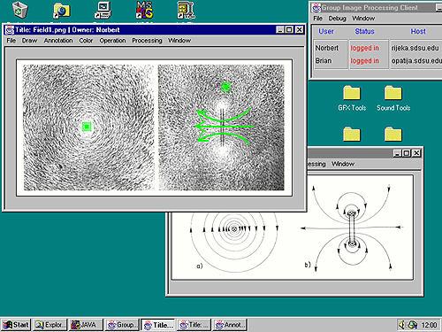
Users can load images into the session at any time. Those images are shared objects, meaning that they are visible and accessible by all session members. Every newly loaded image is displayed in a special image window. Figure 2.3 shows an example session with two loaded images. The title bar of the image window displays the name and the owner of the image. A number of image-related operations can be selected from the image window's menu system. The available functions are grouped into general functions, drawing functions, annotations, color manipulation, geometrical transformations and image processing. Changes made to the image are immediately visible to all session members. Note that only the creator of the image, e.g. the user who loaded the image, and super users can manipulate the image.

  

Figure 2.4: Screenshot of two image windows.

2.4.1 General Image Functions

The user can execute the following operations selectable from the File menu:

• Undo: This removes the last performed image or drawing operation. Activating this function twice will bring back the prior condition again.

• Clone Image: This creates a new image window, which contains a replica of the current image. The image as well as the drawings and annotations are also copied. The user who executed this command will become the owner of the cloned image. This function can be used if a user wants to manipulate an image, which is not owned by the user. The desired image operation can be performed on the clone instead. Sometimes it is also useful to clone an image before a number of sequential changes are carried out and when it is not certain if they will yield the desired effect. The undo function can only remove one operation at a time. In this case, the better choice is to clone an image before some major changes are made.

• Load image: Loads an image and opens a new image window to display it. The image file formats GIF, JPG and PNG are supported.

• Load Image from URL: The user is asked to enter the URL of the image that should be loaded. The new image is again added to the session and displayed within a new image window. This function allows downloading of GIF and JPEG images from any accessible web site.

• Save Image: Saves the image as a file to the local file system. The image can be saved in one of the file formats GIF, PNG, PPM or JPG. Before the image is actually saved the user is asked to select one of three saving modes (see figure 2.5). The default option is to save the plain image alone. However, it is also possible to save the image together with its drawings or to save the drawings alone without the underlying image. Note that drawings that are saved together with the image become a permanent part of the saved image. They can no longer be removed easily from the image. Sometimes it is more appropriate to save the drawings separately (see drawing commands, section 2.4.2). In that case the drawings stay in their vectorial form and can still be modified and removed later.

  
  

    

  Figure 2.5: The save-image dialog box.

  
  

• Remove Image: Removes the image including contained drawings and annotations from the session. Only the creator of the image and super users can execute this command.

• Exit session: The user is leaving the session by selecting this command. He can however log into the session again later on. All his access rights will be restored, e.g. objects created by him will still belong to him.

   
2.4.2 Drawings

Drawings can be used by participants to make corrections within the image or to emphasize and mark up regions of interest. The drawing functions are useful in many situations. For example, a user wants to show the fastest way from point A to point B on a map. Or an electronic circuit is displayed and some users want to make corrections, e.g. cross out wrong parts and insert new ones. Perhaps students wish to study an x-ray image and need to circle in anomalies. The laboratory provides a generic set of drawing shapes, which should be sufficient for most situations.

  

Figure 2.6: Examples of possible drawing shapes.

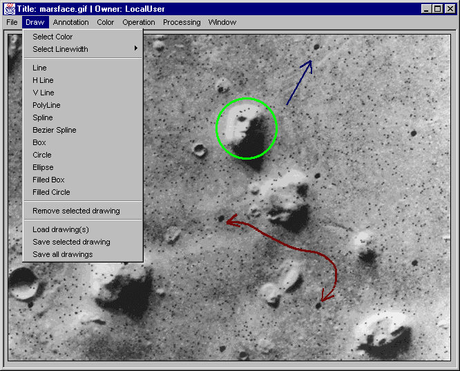
A drawing, which was just made by a user, is immediately visible to other users. Every user can select a color in which the drawings are painted. Drawings created by different users can be differentiated in that way. All drawings are displayed in a separate layer above the image. Supported shapes, selectable from the draw menu, are lines, horizontal and vertical lines, polylines, approximated and interpolated cubic curves, boxes, circles, ellipses, filled boxes and filled circles (see figure 2.6). The line width of a shape can be specified in a range from one to eight pixels. Lines and curves can be drawn plain or with an arrow on one or both ends.

All types of drawings are created in the same way, by specifying a number of control points that define the drawing. As an example, let's say we want to draw a line. First, the menu command Line must be selected from the draw menu. Then the starting point of the line is set by clicking at the desired position within the image. A small box that marks the beginning of the line appears on the screen. The point can be moved around while the mouse button is held down. Once the mouse button is released, the point is frozen to its latest position. The same procedure has to be repeated to define the end point of the line. The line is displayed and can be changed by moving the end point around with the pressed mouse button. The line is finished once the mouse button is released.

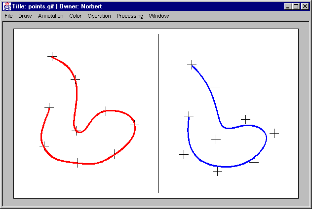
Every supported shape is defined according to this procedure. The drawing is finished once its last control point has been set. Some figures, curves and polylines for example, have an unspecific number of control points. Those drawings are finished by clicking on the right mouse button once all necessary points have been specified. Figure 2.7 shows an example of two curves and their control points. A completed drawing can be selected by clicking on it. It can also be moved around within the image by dragging it with the mouse.

  

Figure 2.7: Comparison of an interpolated and an aproximated curve drawn according to an identical set of control points.

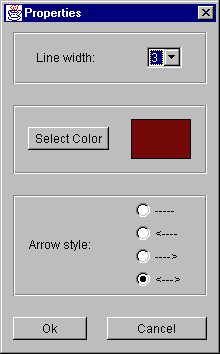
A special property window is displayed by double clicking on a drawing (see figure 2.8). This window can be used to change attributes of a drawing. Common attributes, which can be altered for all types of drawings, are the line width and the color. Lines and curves can also have arrows on one or both endings. This can be adjusted in the arrow style area. This area is not displayed for boxes, circles and ellipses.

  

Figure 2.8: The drawing property dialog box.

Drawings can be removed as well as stored and reloaded. This is done by selecting a drawing, i.e. clicking on it, and by choosing the appropriate command form the draw menu. Here is a summary of functions available from the draw menu:

• Select Color: A color selector dialog will be displayed, which can be used to select a desired color. All further drawings will be drawn in the selected color.

• Select Line Width: Allows user to change the default line width by selecting a line in the range of 1 to 8. Newly created drawings will be painted with this line width.

• Remove Selected Drawing:This removes the currently selected drawing. Note that only super users and the creator of the particular drawing can remove the selected drawing.

• Save Selected Drawing: Stores the selected drawing to a local file. The file must be specified via a file dialog box.

• Save All Drawings: This is similar to the previous command, except that all drawings of that image are saved together to a local file.

• Load Drawing(s): Restores previously saved drawing(s) from a file. The file is selectable via a file dialog box. The user who has loaded a drawing automatically becomes the owner of it.

2.4.3 Annotations

An annotation is a text message that can be attached to a desired position of an image. Annotations can be used to make comments about certain features of the image or to leave notes for other users. This is especially useful if a session is carried out over a longer time, e.g. if it is stored and reopened at a later time or date. For example, the annotations can be used as reminders about what has been found out or what has to be done. An annotation is owned by the user who created it. Other users can however add further comments to the annotation.

Annotations can be set at any position of the image. They are displayed as small squared icons. An annotation can be created by selecting Set Annotation from the Annotation menu. It is then required to click on the position within the image where the annotation should be placed. A special annotation window will be opened in which the annotation text must be entered.

  

Figure 2.9: The annotation icon and the annotation window.

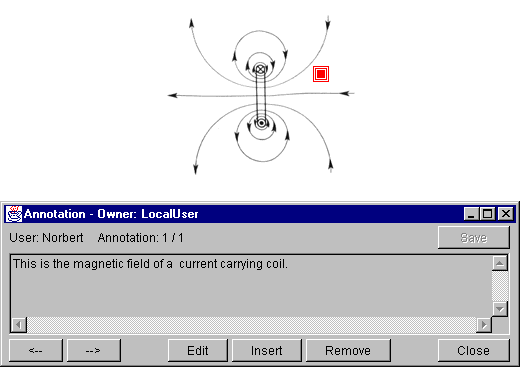
Clicking on Save sets the annotation and closes the annotation window. The annotation icon is now visible to all session members. Figure 2.9 shows an annotation window and an area of an image that contains the corresponding annotation icon. Every session member can read the annotation by double clicking on the annotation icon. This opens the annotation window^2.3. He or she can also add further comments to that annotation. Clicking on `Insert' adds an empty text message behind the currently displayed message. The new message can now be entered. It does not become visible to other users unless it is saved. The number of text messages within the annotation is displayed in the top area of the annotation window. The author of the currently displayed message is also shown. The left and right arrow buttons can be used to scroll through the set of comments. Text messages can also be edited, but only by the author of the particular text message. The annotation menu provides further commands to remove, as well as save and load the whole annotation. The removal of the complete annotation is only allowed by its creator or by super users.

2.4.4 Geometric Transformations

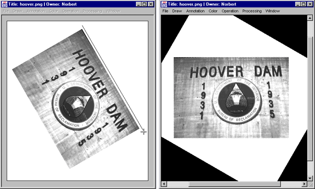
Geometric transformations are applied on the whole image. Supported transformations are scaling, rotating, clipping and mirroring. Figure 2.11 shows an example where an image has been rotated. Note that drawings and annotations are included by the transformation process. The current version of the laboratory determines the resulting pixels by a nearest neighbors algorithm (see section 4.3.3.3). The following geometrical transformations are selectable from the Operation menu:

• Scale: A dialog box will be displayed (figure 2.10), which allows the user to specify the desired dimensions of the image. This can be the size in pixels, or the relative size in x- and y-direction in percent relating to the current size of the image. The image will be enlarged or reduced according to the given values. The width/height aspect ratio can be kept constant by checking the constant aspect check box.

  
  

    

  Figure 2.10: The scale dialog box.

  
  

• Rotate: This function can be used to rotate the image. For example, scanned images often need to be rotated because the scanned document was not lined up correctly. After selecting Rotate from the operation menu, the degree of rotation must be defined by specifying the direction of the desired horizontal axis. This is done by using a rubber band that represents the new imaginary horizontal axis. Clicking on a point in the image sets the starting point of the rubber band. The mouse button must be held down and can be moved around. The rubber band will be visible in form of a straight line between the starting point and the current position of the mouse pointer. The mouse button can be released once the rubber band has been lined up in the desired direction. The image will now be rotated according to the specified direction of the horizontal axis. Figure 2.11 shows an example of an image which needs to be rotated. The left figure shows how the user is specifying the new horizontal axis by lining up the rubber band with the edge of the image. The right figure shows the resulting image after rotation.

  
  

    

  Figure 2.11: An image before and after rotation.

  
  

• Clip: Sometimes, a picture contains unwanted borders or only a certain part of the image is relevant. This function allows the user to clip an image according to a predefined clipping box. The upper left corner of the clipping box must be specified by clicking on the desired position. The clipping box appears and can be adjusted by dragged the lower right corner of the clipping box while holding the mouse button pressed. The borders outside of the clipping box will be removed once the mouse button is released. Figure 2.12 shows the example image from figure 2.11 after is has been clipped.

  
  

    

  Figure 2.12: A clipped image.

  
  

• Mirror X or Mirror Y: Those functions mirror the image relative to the X or Y axis. This is sometimes useful in situations where a transparent photo slide has been scanned from the wrong side, or if the scanned or loaded picture is upside down.

2.4.5 Image Processing

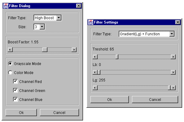
The distributed graphics laboratory allows the user to process images by applying mask filter operations. A mask filter alters each pixel's intensity based on its current value and the intensity of the neighboring pixels. Two groups of filters are available, which can be selected from the Processing menu. Selecting Mask Filters displays the mask filter dialog box (see figure 2.13a), in which the desired filter operation can be chosen and configured. Selecting the menu entry Gradients displays the gradient dialog box (figure 2.13b). This dialog box allows the user to choose from a set of gradient operations.

  

Figure 2.13: The mask filter and gradient filter dialog box.

The next two sections describe how the supported filter types are used. More detailed information about the implemented filters can be found in section 4.3.3.

2.4.5.1 Mask Filter

The mask filter dialog consists of three parts. The desired filter type and mask size can be selected in the top area. The filter functions Low Pass, High Pass, High Boost and Median are currently supported. The dimension of the filter mask can be one of the sizes 3, 5, 7 or 9. The center area is only applicable for the High Boost Filter. The slider in this area must be used to set the desired boost factor, which can be in the range from 1.0 to 2.0. The bottom part of the dialog box contains control fields that influence how the filter is dealing with color images. By selecting Grayscale Mode, the image will be converted into gray-scale before the filter is applied. It is also possible to preserve the color information by selecting Color Mode. In this case, the filter operation is performed separately on the intensity levels of each pixel's color components red, green and blue. Of course, this takes three times longer then gray-scale filtering if all three color channels are selected.

  

Figure 2.14: Examples of several mask filter operations.

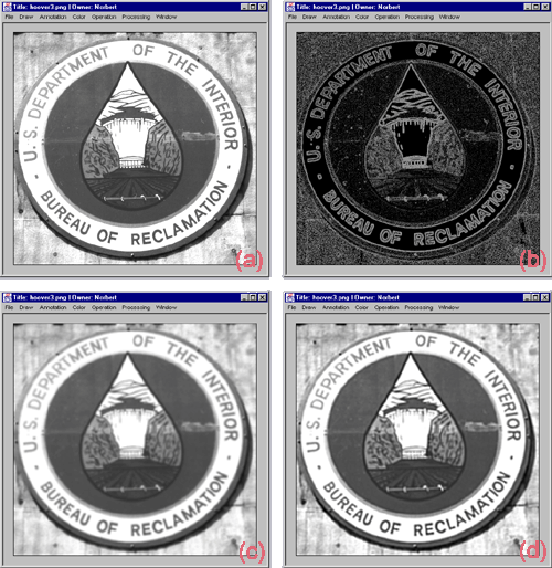
Figure 4.11a shows an example image that is used to demonstrate the different effects of several filter types. Figure 4.11b is shows the example after filtered with a 3x3 high pass filter and figure 4.11c is shows the results when filtering the same image with a 5x5 low pass filter. The low pass filter is blurring the image, which means that the low frequency components have been suppressed. Such filters can be used to reduce noise or to smooth digitized images with a low number of planes. Note that the median filter (not shown in the examples) can also be used to remove noise. The median filter is, in most cases, the better choice for noise removal. This is especially the case for spike like noise. The high pass filter does the opposite when compared to the low pass filter. It eliminates the high frequency terms, which can be can be seen in figure 4.11b. Only the edges of the image remain. Finally, figure 4.11d shows the attempt to sharpen the low pass filtered image from figure 4.11c by applying a 9x9 high boost filter with a boost factor of 2.0. Although the resulting image is still slightly blurred, it is noticeably sharper then the image from figure 4.11c.

2.4.5.2 Gradient Filter

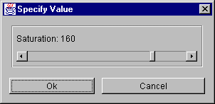
The gradient filter produces a grayscale image, whose pixels represent the gradients^2.4 of the corresponding pixels in the initial image. This operation is performed by selecting Gradient as filter type in the gradient dialog box. There are however four additional types of filters. They perform further thresholding operations based on the output of the gradient filter. The results of those filter operations depend on adjustable parameters in the bottom part of the gradient dialog box (see figure 2.13b). The following table gives a summary of selectable filter types. It also explains how the results are influenced by the parameter threshold and the two adjustable gray values Lg and Lb:

Type	Function
Gradient	No thresholding is performed. A pixel in the resulting image represents the gradients of the corresponding pixel in the initial image.
Gradient + Function	Only pixels, whose gradient is greater or equal to the selected threshold, are replaced by the gradient. All other pixels stay unchanged.
Gradient(Lg) + Function	Pixels, whose gradient is greater or equal to the threshold, are replaced by the gray value Lg.
Gradient + Function(Lb)	Pixels, whose gradient is greater or equal to the threshold, are replaced by their gradient. All other pixels are set to gray value Lb.
Gradient(Lg) + Function(Lb)	Pixels, whose gradient is greater or equal to the threshold, are replaced by gray value Lg. All other pixels are set to gray value Lb.

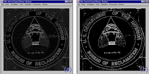
Figure 2.15 shows two images that have been produced by different types of thresholding. The left image shows the result of applying the plain gradient filter on the example image from figure 4.11a. The right image shows the result by using the filter type Gradient(Lg) + Function(Lb) with a threshold of 65, Lg set to 0 and Lb set to 255. Pixels, whose gradient is below 66, have been set to black. All other pixels appear in white.

  

Figure 2.15: Gradient filtered images produced with different types of thresholding.

2.4.6 Color Manipulation

The color menu provides a set of functions that deal with the processing of the image's color information. The following functions are available from the color menu:

• Convert to Black and White: This operation reduces the number of colors to two. Before the conversion is executed, the user is asked to give a threshold, which must be a value between one and 256. Pixels, whose intensity is below this threshold, are replaced by black pixels. All other pixels are set to white.

• Convert to Gray Scale: This converts the image into grayscale.

• Set Saturation: This operation can be used to change the color saturation of the image. The desired saturation must be specified with a special dialog box shown in figure 2.16. The selected value can range from 0% to 200%. A value of 200% would double the saturation of every pixel. A value of 0% would convert the image into gray scale.

  
  

    

  Figure 2.16: The saturation dialog box.

  
  

• Histogram: The histogram of an image graphically represents the statistical distribution of occurring pixel intensities. Selecting the histogram function from the color menu will open a histogram window as shown in figure 2.17. In case of a gray scale image, this window will only show one histogram, which displays the distribution of the 256 possible gray levels. For color images, this window displays the histogram of the intensity levels. Further, it contains three additional histograms for the color intensities of the components red, green and blue. Two operations, histogram equalization and histogram specification, can be carried out from within the histogram window.

  
  

    

  Figure 2.17: Histograms of a color image displayed in the histogram window.

  
  

2.4.6.1 Histogram Equalization

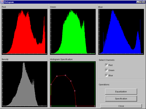
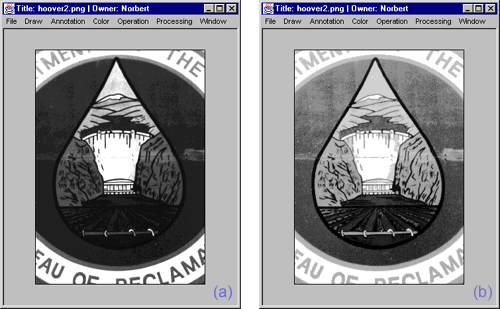
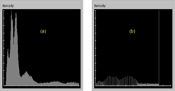
Histogram equalization is an operation that remaps the pixel intensities of an image in such a way that the histogram becomes equally distributed. This can be used to enhance too dark or too bright images or images with low contrast. Figure 2.18a shows an image, which appears very dark. Figure 2.18b contains the same image after histogram equalization. It can be seen that many details are now visible that were not noticeable in the original image. Figures 2.19a and 2.19b show the histograms of the image before and after equalization. Note that the implemented histogram equalization algorithm is only calculating an approximation. In an ideal case, the histogram is completely flat (equally distributed). The results are however qualitative sufficient, because subtotals over equally spaced areas of the histogram produce identical sums. See section 4.3.3.5 for a detailed description of the implemented algorithm.

  

Figure 2.18: An image before and after histogram equalization.

  

Figure 2.19: The histograms before and after histogram equalization.

2.4.6.2 Histogram Specification

Histogram equalization is used to produce an equally distributed histogram. With histogram specification however, it is possible to specify a specific histogram shape. The intensity levels of the image will be remapped so that the new histogram is equal to the specified histogram shape.
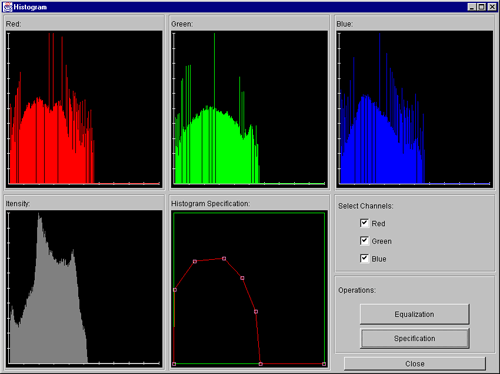
In the graphics laboratory, the desired histogram shape can be specified in the lower left area of the histogram window (see figure 2.17). The shape can be changed by moving the control points with the mouse. Once the desired shape has been defined, the conversion process can be started by clicking on Specification. Figure 2.20 shows the histogram after the performed histogram specification. It should be noted that the implemented algorithm is again only producing an approximation of the given shape.

  

Figure 2.20: The histogram after histogram specification.